Our understanding of how molecular clouds form in the interstellar medium (ISM) would be greatly helped if we had a reliable observational tracer of the gas flows responsible for forming the clouds. Fine structure emission from singly ionised and neutral carbon ([CII], [CI]) and rotational line emission from CO are all observed to be associated with molecular clouds. However, it remains unclear whether any of these tracers can be used to study the inflow of gas onto an assembling cloud, or whether they primarily trace the cloud once it has already assembled. In this paper, we address this issue with the help of high resolution simulations of molecular cloud formation that include a sophisticated treatment of the chemistry and thermal physics of the ISM. Our simulations demonstrate that both [CI] and CO emission trace gas that is predominantly molecular, with a density n ~ 500-1000 cm$^{-3}$, much larger than the density of the inflowing gas. [CII] traces lower density material (n ~ 100 cm$^{-3}$) that is mainly atomic at early times. A large fraction of the [CII] emission traces the same structures as the [CI] or CO emission, but some arises in the inflowing gas. Unfortunately, this emission is very faint and will be difficult to detect with current observational facilities, even for clouds situated in regions with an elevated interstellar radiation field.
Clark, Paul C.; Glover, Simon C. O.; Ragan, Sarah E.; Duarte-Cabral, Ana
2018, ArXiv e-prints, 1809, arXiv:1809.00489
http://adsabs.harvard.edu/abs/2018arXiv180900489C
Context
At the present time, the most favoured models are ones in which clouds form from converging flows of atomic or molecular gas, driven either by stellar feedback processes (supernovae, stellar winds etc.), or by large-scale gravitational instability. However, observational evidence in favour of either of these pictures remains scarce. One reason for this is the difficulty involved in finding good observational tracers of the cloud assembly process. The most commonly used observational proxy for H2 is carbon monoxide, CO. Unfortunately, although this molecule is an extremely useful probe of the behaviour of H2 within molecular clouds that have already formed, it does not appear to be a good tracer of the cloud assembly process. Most clouds that are CO-bright are associated with at least some level of ongoing star formation, suggesting that they have already accumulated enough mass to become gravitationally unstable.
One promising alternative is the use of the [CII] 158 μm fine structure line as a tracer of CO-dark molecular gas. Both observations (Pineda et al. 2013) and simulations (Glover & Smith 2016) suggest that a significant fraction of the observed emission originates from H2-dominated gas. Nevertheless, the reliability of [CII] emission as a tracer of molecular gas on the scale of individual molecular clouds remains to be established.
Another possibility is neutral atomic carbon, C, which has two fine structure lines at 370 μm and 609 μm. Chemically, C is found in regions intermediate between the lower density, low extinction material traced by [CII] and the higher density, high extinction gas traced by CO. It is therefore more effective than CO at tracing gas at the boundaries of molecular clouds (Glover et al. 2015).
Simulations of [CI] emission from realistic molecular clouds have so far focussed on clouds that have already formed, and hence have been unable to explore whether [CI] is a good tracer of the inflowing gas, or whether, like CO, it primarily traces the cloud once it has already assembled.
Goal of the paper
Their goal is to determine what regimes the various tracers can probe – in terms of density, temperature and molecular (H2) fraction – and how this varies as the clouds are exposed to progressively stronger interstellar radiation fields (ISRFs) and cosmic ray ionisation rates (CRIRs).
They focus on the emission from 4 lines: [CII] 158 μm, CO (1-0) and the first two lines of [CI] : the 3P1 →3 P0 transition at 609 μm and the 3P2 →3 P1 transition at 307 μm
Numerical setup
Code : AREPO (MHD; simplified treatment of the chemical and thermal evolution) + NL99 for chemistry (Glover & Clark 2012) and TREECOL to compute dust extinction and molecular shielding.
Initial conditions : collision of two atomic clouds (n=10cm^-3, 10^4 Msol, R=19pc). The initial clouds are CNM (abundance of H2 is zero).
Each cloud has a turbulent velocity dispersion of 1 km/s with P(k) ~ k^-4 with only solenoidal modes. The two clouds collide with a velocity difference of 7.5 km/s. They impose a uniform magnetic field of 3 microG, parallel to the collision direction. The two clouds are embedded in WNM gas (n=0.1 cm^-3) in a box of 190pc. Their spatial resolution depends on local density but is ~0.1 pc or better where C and CO is present.
They stop the simulation when the first prestellar core is gravitationally unstable (no feedback in their simulation).
They did 3 simulations of this type with different ISRF (1.7, 5.1 and 17 times Habing) and CRIR (0.3, 0.9 and 3 x 10^-16 s^-1). They vary them together to mimic the effect of nearby star-forming events.
They interpolated the AREPO simulation on a cartesian grid (0.024 pc resolution) and then use RADMC-3D to do the radiative transfer. They use dv = 0.020 km/s to build the synthetic observations.

HI-H2 transition
All their simulations resulted in the formation of a network of dense molecular (i.e. H2-rich) structures, with around 50% of the initial hydrogen mass being converted to molecular form by the point at which they stop the simulations. The amount of molecular gas formed has little dependence on the strength of the ISRF or the CRIR.
The gas makes the transition from H to H2 at around a number density of a few 100 cm−3, irrespective of the CRIR and the strength of the ISRF. However the carbon chemistry changes occur at much higher densities. For the solar neighbourhood ISRF and CRIR, C+ is still the dominant form of carbon at a number density of 1000 cm−3, and CO does not become dominant until a density of nearly 10^4 cm−3. When the ISRF and CRIR are 10 times higher, these transitions are shifted up in density by a factor of ∼5. At no point is the neutral form of carbon the dominant form.
Density regime of each tracer
They have seen that the [CII] traces a different regime to the [CI] and CO, probing gas that is of lower density, slightly higher temperature and of mainly atomic, rather than molecular, composition. The majority of the [CII] emission comes from gas with number densities ∼ 100 cm−3, which is still predominantly atomic in nature. At higher densities the gas is too cold to excite the line, and at lower densities the emissivities are too small to be readily detectable with current observing platforms. However, they note that gas at this density has not yet reached chemical equilibrium in their simulations, and it is therefore plausible that if they were to examine much older clouds, they would find a much larger fraction of the [CII] emission coming from H2-dominated gas.
Using the Herschel GOT C+ survey of [CII] emission in the Galactic plane, together with HI, CO and star formation tracers, Pineda et al. (2013) found that in the Milky Way, only around half of the observed [CII] emission is directly associated with star-forming clouds, with most of this emission coming from dense photodissociation regions (PDRs) and a small fraction from HII regions. The other half of the observed [CII] emission arises in gas clouds illuminated by relatively weak radiation fields (G0 = 1–10). Pineda et al. (2013) also concluded that roughly 60% of the [CII] emission that is not directly associated with star formation comes from H2-dominated clouds, with the remainder coming from clouds dominated by atomic gas.
An age effect
In their simulations, Clark et al. (2018) found that a large fraction of the [CII] emission comes from gas dominated by atomic hydrogen, and only a small fraction comes from gas dominated by H2 (France et al. 2018 found a similar result). Part of the reason may be the under-correction for HI optical depth by Pineda et al. (2013). The authors suggests that it might be a consequence of the evolutionary state of the clouds. The gas clouds sampled in the GOT C+ survey may have a wide range of ages as the clouds simulated here are young. Given the relatively long formation timescale for H2 at densities below n ∼ 100cm−3, it is likely that the gas producing the bulk of the [CII] emission in the simulations has not yet reached chemical equilibrium, and that older clouds may produce more of their [CII] in H2-dominated gas and less in HI-dominated gas. Interestingly, using a simulation with clouds with a broader range of dynamical ages, Glover & Smith (2016) found that roughly half of the [CII] emission in their model comes from H2-dominated gas, with the remainder coming from H-dominated gas.
Velocity dispersion
the σmom−2 for the [CII] line is generally higher than that from both [CI] and CO lines. These differences must be due primarily to differences in the bulk motions of the gas traced by the different forms of emission. They don’t think this is the effect of thermal broadening being stronger for [CII]. Support for this conclusion comes from the fact that we see only relatively minor differences in σmom−2 in the runs with different ISRF strengths and CRIRs, despite the substantial differences in the temperature structure of these two runs.
They also see that σmom−2 for CO and [CI], rises with increasing column density. This is interesting, since it goes in the opposite direction to the “transition to coherence” picture that is often claimed for pre-stellar cores in molecular clouds (see e.g. Goodman et al. 1998, Kirk et al. 2007, J. E. Pineda et al. 2010), although this transition is generally seen in high density tracers such as N2H+ or NH3, rather than [CI] or 12CO. The fact that the bulk of the CO emission is coming from gas around a few 1000 cm−3 – around the critical density – means that the line-width of any given parcel of emitting gas will be only 0.2 km s−1, the sound speed at around 10 K. That we see σmom−2 > 0.2 km s−1 implies that we are seeing non-thermal contributions from multiple parcels of gas along the line-of-sight. There are two reasons why σmom−2 would then increase with increasing column density. The first is that higher column density regions can be the result of more violent compression, and so what we are seeing is the residual velocity components that have survived the shock. Only head-on collisions in uniform flows would result in a post-shock velocity of zero, and even then, only if the gas remains thermally stable; oblique shocks will always have left over shear, the amount of which will scale with the with strength of the shock, which also increases the density of the gas. The second reason that we see a higher σmom−2 with increasing column density could simply be due to the additional influence of gravity as we go to progressively denser structures.
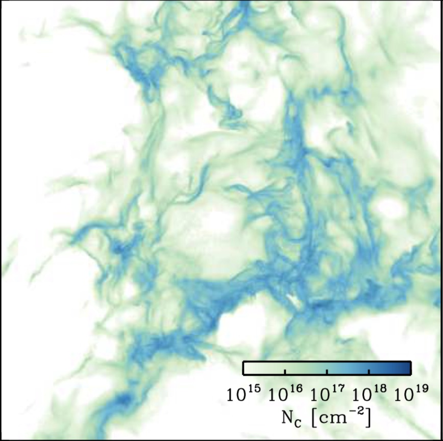
It is also interesting that the behaviour seen in Figure 6 is the opposite from what we see in Figure 1, where the density-weighted velocity dispersion in the regions of high-column is markedly lower than that found in the regions of high density. Given that we expect line emission to scale linearly with density in the LTE regime and with the density squared for sub-thermal excitation, this is clearly a worry for our observational interpretation of the gas velocities in molecular clouds. Indeed, it suggests that a more careful decomposition of the line emission data is required to make sense of the kinematics, such as the technique presented in Henshaw et al. (2016).
MAMD : another explanation, not mentioned by the authors, is that larger column density corresponds to structure that are longer on the line of sight (or the sum of several structures) which, given the turbulence velocity scaling with size, would lead to larger velocity dispersion. In other words, $N=n \times L$, so an increase of N could be either an increase of n (the case they mention) or an increase of L.
