We carried out synthetic observations of interstellar atomic hydrogen at 21 cm wavelength by utilizing the magnetohydrodynamic numerical simulations of the inhomogeneous turbulent interstellar medium. The cold neutral medium (CNM) shows a significantly clumpy distribution with a small volume filling factor of 3.5%, whereas the warm neutral medium (WNM) has a distinctly different and smooth distribution with a large filling factor of 96.5%. In projection on the sky, the CNM exhibits a highly filamentary distribution with a subparsec width, whereas the WNM shows a smooth, extended distribution. In the H I optical depth, the CNM is dominant and the contribution of the WNM is negligibly small. The CNM has an area covering factor of 30% in projection, while the WNM has a covering factor of 70%. This means that the emission-absorption measurements toward radio continuum compact sources tend to sample the WNM with a probability of 70%, yielding a smaller H I optical depth and a smaller H I column density than those of the bulk H I gas. The emission-absorption measurements, which are significantly affected by the small-scale large fluctuations of the CNM properties, are not suitable for characterizing the bulk H I gas. Larger-beam emission measurements that are able to fully sample the H I gas will provide a better tool for that purpose, if a reliable proxy for hydrogen column density, possibly dust optical depth and gamma rays, is available. The present results provide a step toward precise measurements of the interstellar hydrogen with ˜10% accuracy. This will be crucial in interstellar physics, including identification of the proton-proton interaction in gamma-ray supernova remnants.

Fukui, Yasuo; Hayakawa, Takahiro; Inoue, Tsuyoshi; Torii, Kazufumi; Okamoto, Ryuji; Tachihara, Kengo; Onishi, Toshikazu; Hayashi, Katsuhiro
2018, The Astrophysical Journal, 860, 33
http://adsabs.harvard.edu/abs/2018ApJ…860…33F

Numerical setup

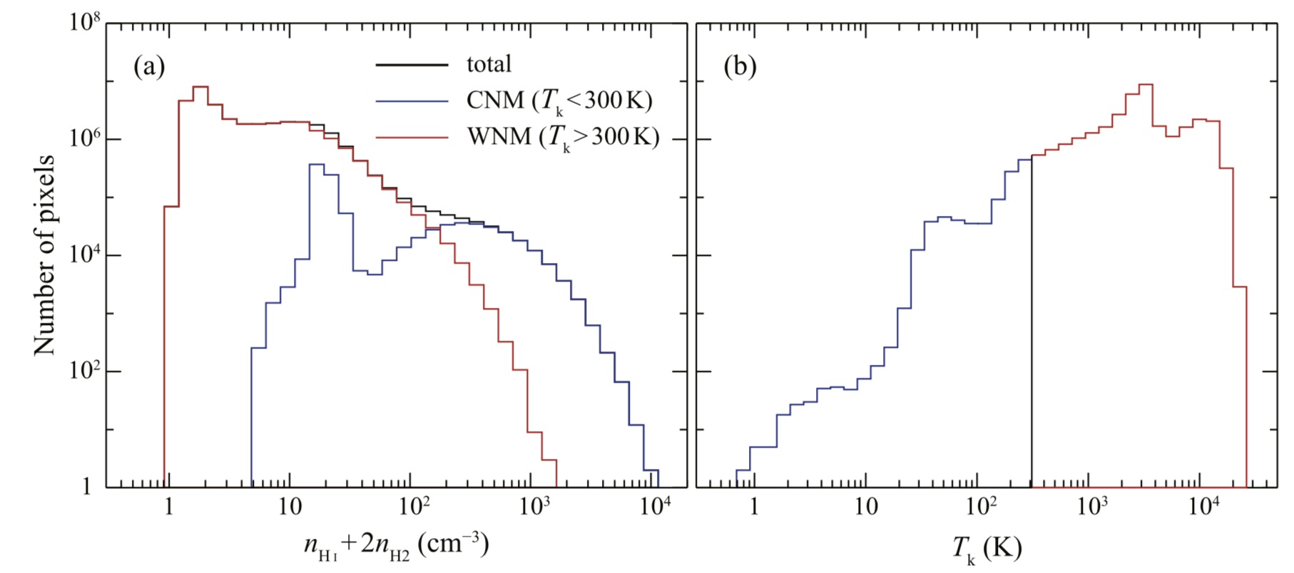
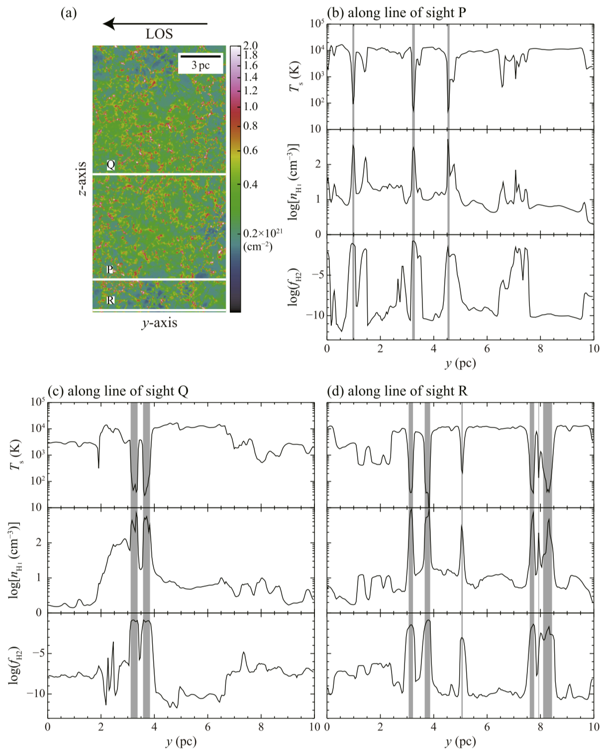
These simulations deal with converging H I flows as a function of time over 10 Myr. The gas is originally H I, while formation of H2 molecules is incorporated by using the usual dust surface reaction. The results indicate two phases of HI, the CNM and the WNM, as well as time-dependent transient gas, which behaves intermediately. In the following, we call for convenience the gas with Ts below 300 K the CNM and that with Ts above 300 K the WNM.

The simulations assume converging H I gas flows at 20 km/s that are initially in pressure equilibrium with the standard interstellar H I having pressure of $p k^{-1} =5.2 \times 10^3$ K cm$^{-3}$. The H I gas flow is inhomogeneous and continuously enters the box from the two opposite boundaries of a cube of (20pc)^3. Formation of molecules such as H2 formation on dust surfaces and CO formation via CH+ with the effects of self/dust UV 2 shielding are taken into account, and radiative and collisional heating and atomic and molecular cooling are incorporated.

Size of simulation is 1024^3 but they worked with a degraded version of 512^3 to reduce the data size. In this reduced version, the pixel size is 0.04 pc.
Simulations runs for 10 Myr.
The gas mass increases with time.

For their analysis they extracted lines of sight with WHI > 150 K km/s (corresponding to 2.7E20 cm^-2). For a box of 20pc deep, this is corresponds to an average density of 4.6 H/cm^-3

Figure 1. Volume rendering map of spatial distribution of pixels with Ts<300 K (black) and those with Ts>300 K (gray) in the 0.5 Myr model. The red contour projected on the front surface outlines the region of interest (ROI). The pixels outside of the ROI are blanked and not used in Figures 2, 4(a), 5, 10, 11, 13, 15 and Table 3.

Results

Figure 5. Histograms of (a) total hydrogen density (nHI+2nH2) and (b) kinetic temperature (Tk) for each pixel in the 0.5 Myr model. The blue lines represent the contribution of TK<300 K, and red lines represent that of TK>300 K.

Figure 5. (c) Probability distribution function in the nH I–Tk plane. The contours have equal logarithmic spacing. The straight distribution in the lower right shows the initial H I flows prior to the collision.

Figure 6. (a) Side view of the H I column density in the y–z plane integrated in the x direction in the model. Three lines of sight selected are shown by the lines P, Q, and R (see the text and Table 5). The image is 10 pc × 20 pc in size. The y axis in the numerical domain corresponds to the horizontal axis and the z axis to the vertical axis. (b) Ts, nH I, and H2 fraction fH2=2nH2/(2nH2+nH I) profiles (from top to bottom) along the line of sight P. The horizontal axis is the distance from the far side of the model ISM, y. The CNM spikes are indicated by shaded regions. (c) and (d) Same as (b) but along lines of sight Q and R, respectively.

The authors mention that the ISM compressed by the converging flows in the 0.5–1.0 Myr seems to be the representative state of the dynamic ISM. They justify it by the fact that the ISM is perturbed by a supernovae explosion every 1Myr.

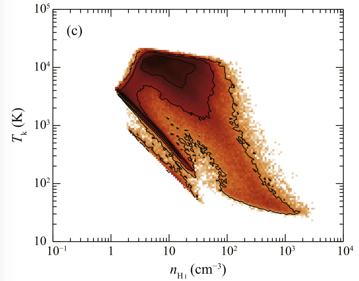
On the other hand, most of the gas seems to be in the thermally unstable regime, probably due to the rather high pressure and high turbulent energy induced by the convergent flow.

Conclusion

In order to gain insight into the detailed physical conditions of the interstellar H I gas and its observed properties in the solar neighborhood, we carried out synthetic observations of the interstellar HI gas at 21cm by using the MHD numerical simulations of the realistic inhomogeneous H I gas that is in the converging flows (Inoue & Inutsuka 2012). The simulations incorporate the microscopic processes including the H2 formation reactions, the magnetic field, and the heating/ cooling. The simulated HI gas is highly turbulent and inhomogeneous and is far from equilibrium with a typical dynamical timescale on the order of megayears. The results were compared with the conventional emission–absorption measurements. The main conclusions of the present study are summarized as follows:

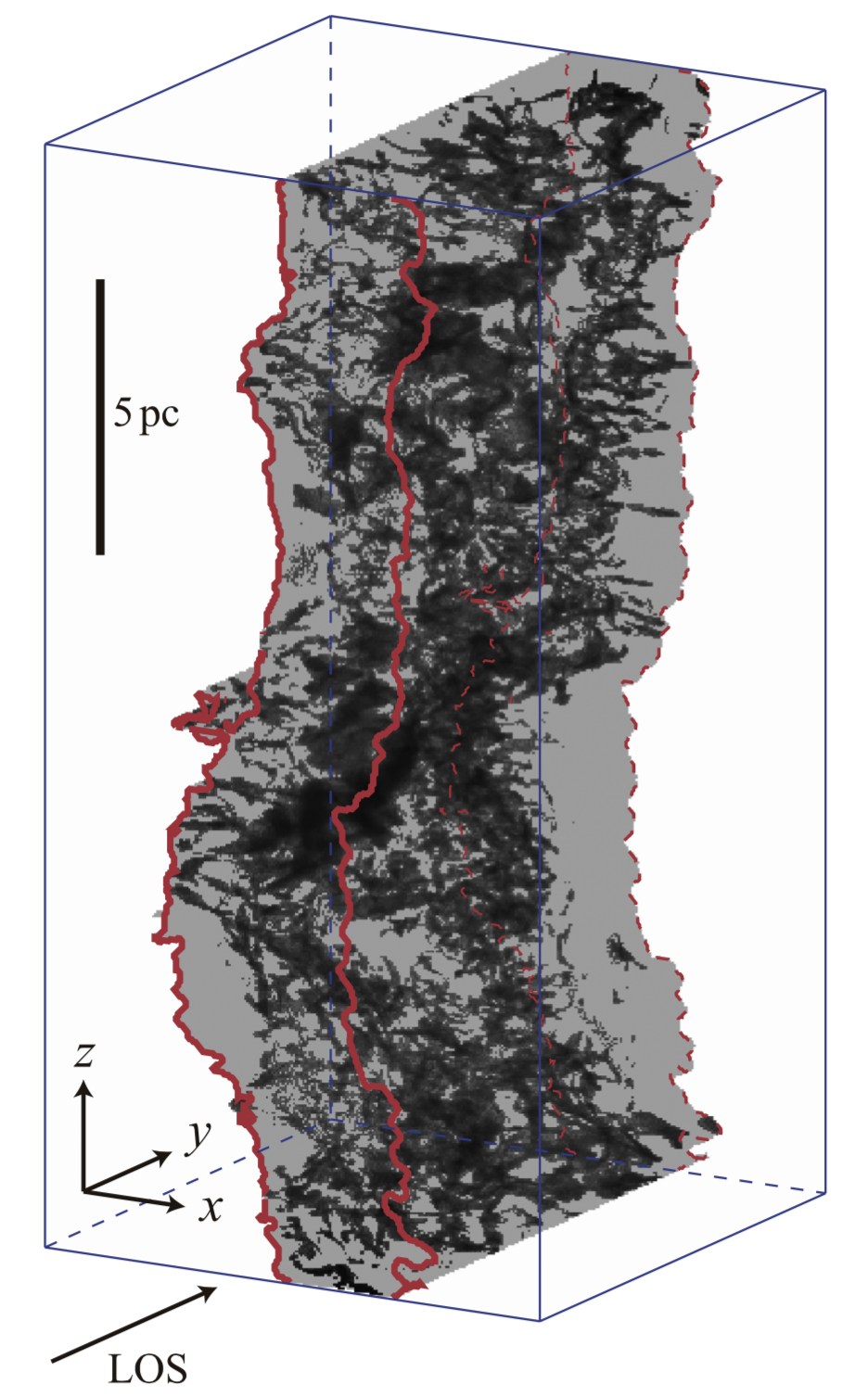
The present analysis was made for the model at an evolutionary epoch of 0.5 Myr, which was chosen from the simulation results covering a time span of 10 Myr. The model reproduces the distribution of the H2 fraction fH2 that is consistent with the ultraviolet measurements of H2. As shown by the previous works over the last five decades, the HI gas consists of two components, the CNM and the WNM. The CNM has a spin temperature Ts ranging from 10 to 300 K, and the WNM has from 300 K to 10,000K. The density range of the CNM is from 10 cm−3 to 10^3 cm−3 and that of the WNM from 1 to 100 cm−3. The synthetic observations show that the CNM has a small volume filling factor of 3.5%, whereas the WNM is distributed with a volume filling factor of 96.5%, while the gas mass of each component is comparable. These filling factors are consistent with the peak density of the CNM being larger than that of the WNM by a factor of ∼30. The CNM distribution is highly clumpy and filamentary with a subparsec size scale, and the WNM distribution is smooth with much fewer small-scale structures. As a result, the CNM covering factor is small, ∼30%, in the sky. These represent general properties of the H I gas in the solar neighborhood.
HI line profiles were calculated by separating the CNM and WNM. The CNM is seen as a narrow feature of ∼5 km/s in half-power full line width and the WNM as a wing-like feature spanning over ∼40 km/s. These properties are consistent with the observed HI profiles, lending support to the chosen model. By setting the background radiation, absorption line profiles toward radio continuum sources were also synthesized. The HI distributions in the sky were reproduced in the 21 cm line integrated intensity (W_HI), the HI column density (N_HI), and the velocity-integrated optical depth ($\tau_{HI}$), for the CNM and WNM separately. Saturation of W_HI due to high $\int \tau_{HI}(V)\,dV$ greater than 2 K km/s is significant in about one-half of the H I gas. This lends support to the optically thick HI presented by Fukui et al. (2015). $\tau_{HI}$ is dominated by the CNM. The contribution of the WNM in $\tau$ is negligibly small due to the $T_s^{-1}$ dependence of the HI opacity.
The properties of the CNM distribution were compared with the observations in a histogram of $\int \tau_{HI}(V)\,dV$. It is notable that the fraction of $\tau_{HI}$ less than 4 K km/s corresponds to 80% of the observed pixels, indicating that the conventional emission–absorption measurements preferentially sample smaller $\tau_{HI}$ of the WNM. This reflects the large covering factor of the WNM. In addition, the nonlinear dependence of $\tau_{HI}$ as (density)$^2$ causes a spatial variation of $\tau_{HI}$ larger than that of $N_{HI}$. The model explains the usual small HI optical depth obtained by the conventional emission–absorption measurements (Heiles & Troland 2003a, 2003b). Conversely, the fraction of $\int \tau_{HI}(V)\,dV$ greater than 2 K km/s is ∼50%, and the real HI optical depth is large enough to cause significant saturation in $W_{HI}$ for about one-half of the total H I mass.
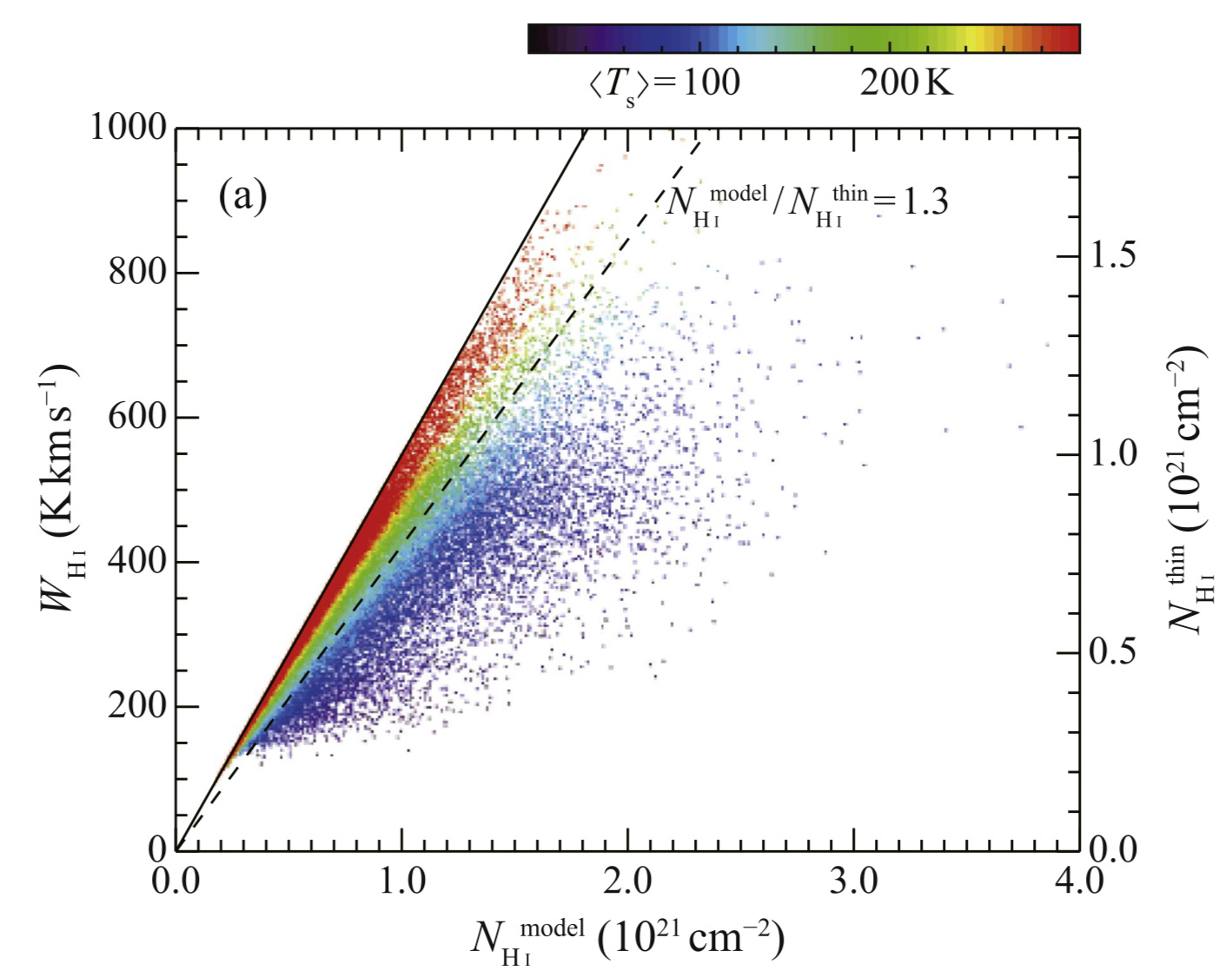
The present model indicates that NH I is close to the optically thin limit within a factor of 1.3 at ∼70% of the observed pixels and within a factor of 1.15 at ∼50% of the pixels. Conversely, pixels with the actual $N_{HI}$ larger than the optically thin case by a factor of 1.3 occupy ∼30% of the pixels. It is usually considered that $N_{HI}$ is consistent with the optically thin limit, whereas the real HI mass of the model is 1.3 times larger than the optically thin approximation. The optically thin approximation thus leads to underestimation of the H I mass by a factor of 1.3, which causes nonnegligible errors in estimating interstellar protons.
A detailed comparison of the model with $N_{HI}$ derived from the conventional emission–absorption measurements indicates that the observed $N_{HI}$ tends to be systematically smaller than $N_{HI}$ in the model by a factor of ∼1.2. It is not entirely clear how $N_{HI}$ was under-estimated in the conventional method. A possibility may be the uncertainty in the contribution of the WNM, whose real intensity is not as accurate as in $\tau_{HI}$.

In summary, we studied the detailed properties of the interstellar HI gas in the solar neighborhood and made it clear that the CNM has significant subparsec structures with a small covering factor in the sky. We showed that the observed quantities in the conventional emission–absorption measurements toward radio continuum point sources are subject to an observational bias toward the WNM having a large covering factor. This bias leads to underestimating $\tau$ and $N_{HI}$. Accordingly, the conventional HI mass must be revised upward by a factor of 1.3 in the present model. The present results provide a step forward toward more accurate determination of the interstellar proton mass. The mass is crucial for identifying the ISM target protons, for instance, in cosmic-ray proton reactions in the gamma-ray SNRs. The results are qualitatively consistent with the Planck/IRAS-based analysis of HI by Fukui et al. (2014, 2015), while a more quantitative pursuit remains as future work, including a test of the nonlinear behavior of the submillimeter dust optical depth due to dust evolution and an extension to the whole sky.