The gases of the interstellar medium (ISM) possess orders of magnitude more mass than those of all the stars combined and are thus the prime component of the baryonic Universe. With L-band surface sensitivity even better than the planned phase one of the Square Kilometre Array (SKA1), the Five-hundred-meter Aperture Spherical radio Telescope (FAST) promises unprecedented insights into two of the primary components of ISM, namely, atomic hydrogen (HI) and the hydroxyl molecule (OH). Here, we discuss the evolving landscape of our understanding of ISM, particularly, its complex phases, the magnetic fields within, the so-called dark molecular gas (DMG), high velocity clouds and the connection between local and distant ISM. We lay out, in broad strokes, several expected FAST projects, including an all northern-sky high-resolution HI survey (22 000 deg2, 3′ FWHM beam, 0.2 km s-1), targeted OH mapping, searching for absorption and maser signals, etc. Currently under commissioning, the commensal observing mode of FAST will be capable of simultaneously obtaining HI and pulsar data streams, making large-scale surveys in both science areas more efficient.
Heiles, Carl; Li, Di; McClure-Griffiths, Naomi; Qian, Lei; Liu, Shu
2019, Research in Astronomy and Astrophysics, 19, 017
http://adsabs.harvard.edu/abs/2019RAA….19…17H
link to PDF file
COSMOLOGICAL EVOLUTION AND THE INTERSTELLAR GAS
Our knowledge of how the Universe has evolved is completely different today from what it was two decades ago. From cosmology and extragalactic astronomy we now have a theory based on cold, dark matter, called DM, that explains with reasonable accuracy the Universe from its first few minutes, through the formation of the first galaxies, to the present era where clusters of galaxies dominate the Universe (e.g. Sommer-Larsen et al. 2003, Komatsu et al. 2009). This theory has been applied in simulations of the Universe that show streams of gas coming together to form the essential building blocks of the Universe, galaxies. These galaxies in turn come alive through bursts of star formation, lose gas to their surroundings and simultaneously accrete new gas to continue their ravenous star formation habit. Eventually after billions of years when their gas supplies run out they cease their star formation, living on perpetually as increasingly red objects filled with low-mass stars.
Thus, the evolution of galaxies is inextricably linked to the interstellar gas, and this is where the models break down. We know that the life cycle of the Milky Way and most galaxies involves a constant process of stars ejecting matter and energy into the interstellar mix, from which new stars then condense, continuing the cycle. For this part of the theory observational or empirical assumptions are inserted, rather than the detailed physics that drives the rest of the models. If we are to understand how galaxies evolve, we must first understand the physics of their evolution in environments we can observe in detail. Our own Galaxy, the Milky Way, provides us with the closest laboratory for studying the evolution of gas in galaxies, including how galaxies acquire fresh gas to fuel their continuing star formation, how they circulate gas and how they turn warm, diffuse gas into molecular gas and ultimately, stars. The Milky Way is a very complex ecosystem. Just as ecosystems on Earth involve many elements linked together by a common source of nutrients and energy flow, the Milky Way ecosystem consists of stars fuelled by a shared pool of gas in the interstellar medium (ISM) and energy that flows back and forth between the stars, the ISM and out of the Galactic disk.
We need to understand the details of these gasdynamical processes that lie at the very heart of the astrophysics. How, exactly, do galaxies form stars, acquire fresh gas, recycle their own gas to form new stars, respond to and dissipate the large-scale energy inputs from supernova and galactic shocks on scales from galactic to sub-parsec. These overarching processes are, in turn, affected by the detailed physical conditions. In particular, these include pressure, temperature, ionization state, magnetic field, degree of turbulence, chemical composition, morphology, and the effects of gravity.
CNM
Our current knowledge of physical conditions and morphology in the CNM depends overwhelmingly on results from the Millennium survey of Heiles & Troland (2005) (HT), who used Arecibo with long integration times suitable for detecting Zeeman splitting. For the HI line in absorption, HT derived column densities, temperatures, turbulent Mach number, and magnetic fields. HI CNM Column densities are usually below 1020 cm$^{−2}$ with a median value N (H I )$_{20} \sim 0.5$. The median spin temperature T$_s \sim 50$ K and the median turbulent Mach number $\sim 3.7$. The median magnetic field $\sim 6 $μG (Heiles & Troland 2005); this is a statistical result and individual detections are too sparse to make a meaningful histogram.
Regarding morphology, Heiles & Troland (2003), in their Section 8, present one of the few discussions of 3-d CNM morphology. By assuming reasonable values for the thermal gas pressure and comparing observed column densities, shapes and angular sizes as seen on the sky, they find that interstellar CNM structures cannot be characterized as isotropic. The major argument is that a reasonable interstellar pressure, combined with the measured kinetic temperature, determines the volume density; this, combined with the observed column density, determines the thickness of the cloud along the line of sight. This dimension is almost always much smaller than the linear sizes inferred from the angular sizes seen on the sky. Heiles & Troland (2003) characterize the typical structures as ‘blobby sheets’, and this applies for angular scales of arcseconds to degrees. An alternative, which they did not discuss, is that the structures are more spherical, but spongelike inside. (If they are spongelike, what fills the holes?) Apart from this general argument, only a very few individual interstellar structures have been characterized morphologically.
The Local Leo Cold Cloud
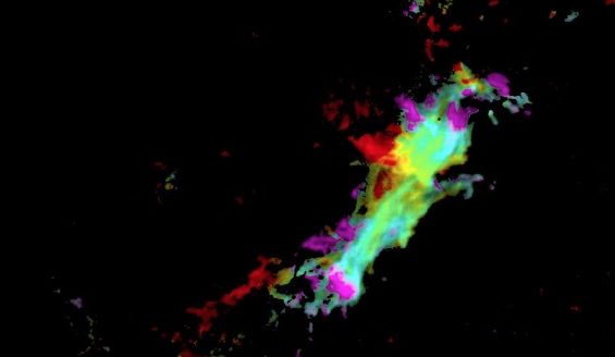
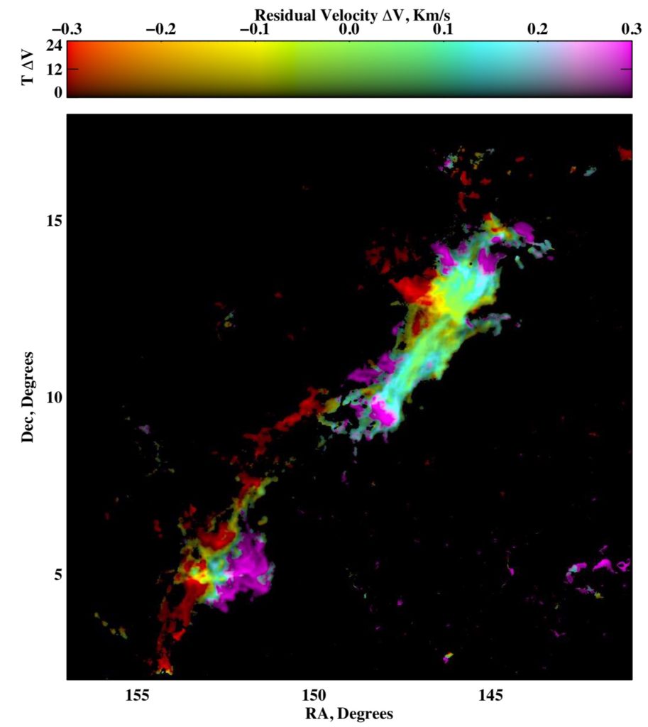
The most spectacular result is the ‘Local Leo Cold Cloud’ (LLCC: Peek et al. 2011a, Meyer et al. 2012), which we characterize as a remarkably thin sheet. Figure 1 images the LLCC, with color indicat- ing the residual radial velocity after subtracting a clear velocity gradient along the length of the cloud, which amounts to about 1 km s$^{−1}$. The cloud temperature, in some places less than 20 K, is measured at a few positions both by emission/absorption of the 21-cm line and by optical/UV spectroscopy. The UV absorption lines of CI provide the interstellar pressure, P/k ∼ 60000 cm$^{−3}$ K, which exceeds the typical interstellar pressure by well over an order of magnitude. The pressure and temperature provide the density, n(HI) ∼ 3000 cm$^{−3}$; the observed column density, N(HI)$_{20}$ ∼ 0.04, provides the thick- ness along the line of sight—about 200 AU. The cloud distance lies between 11 and 24 pc; this close distance, combined with the absorption of diffuse X-rays mapped by ROSAT, confirms the absence of hot gas inside the Local Bubble. With the LLCC’s angular dimension of several degrees, its extent on the plane-of-the-sky is about 1 pc. The aspect ratio (thickness/extent) is about 10$^{−3}$! With a thickness of only 200 AU, the time scale for changing along the line of sight is only a few thousand years— within recorded human history! The $\sim 10$-year time scale for variability of the Na optical absorption line against stars is satisfying confirmation of this rapid evolution (Meyer et al. 2012).
HVC
The nearby HVCs can be used as probes of the thermal and density structure of the Galactic halo. HVCs have, in general, a high velocity relative to their ambient medium, which results in a ram pressure interaction between the cloud and medium. Recent HI observations have indeed shown that a significant fraction of the HVC population have head-tail or bow-shock structure (Bruns et al. 2000). By comparing the observed structures and thermal distributions within them to numerical simulations it is possible to determine basic physical parameters of the Galactic halo such as density, pressure, and temperature. In situations where the density and pressure of the ambient medium are known by independent methods the problem can be turned around to determine the distance to the observed clouds (Peek et al. 2007; Figure 4).
We do not yet have the sensitivity or resolution necessary to study the detailed physical and thermal structure over a large number of HVCs. It seems that the structure that we do see is just the tip of the iceberg. GASS is also revealing a wealth of tenuous filaments connecting HVCs to the Galactic Plane at column densities of N(HI)$\sim 10^{18}$ cm$^{−2}$. As an example, Complex L shows that the HVCs are interconnected by a thin, low column density filament and that this filament appears to extend to the Galactic disk. Filaments of HVCs such as these may be related to the cosmic web predicted in cosmological simulations. Observations of the M31-M33 system (Braun & Thilker 2004, Wolfe et al. 2013) have revealed the local analogue of the cosmic web, showing that very low column density gas (N(HI) ∼ $10^{16} − 10^{17}$ cm$^{−2}$) connects the two galaxies.
Expand the GALFA Survey to an All-Sky FAST-HI Survey
We need to map the 21-cm line over the entire 22,000 deg2 FAST sky—i.e., we need to do with FAST what GALFA did with Arecibo to obtain more sky coverage with the best combination of angular resolution and sensitivity. This will map the ISM morphology generally, including HVCs, and will enhance the sample of the unique structures discovered with GALFA: compact clouds and fibers. This survey should use the multibeam feed for observing efficiency and should cover at least GALFA’s velocity range (±800 km s−1) and resolution (0.2 km s−1). With a resolution of 2.9 arcmin and full sampling (pixel size < 1.5 arcmin) and 12 seconds per pixel, the survey requires about 40000 hours with a single-pixel feed. With the 19-element feed in drift-scan mode, this is a 5000 hour project.